Point Clouds Processing and Interpretation
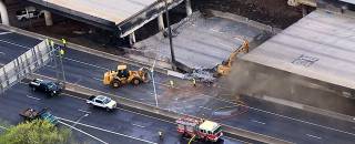
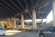
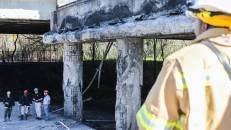
Recently, a section of the I-85 in Atlanta collapsed due to a human-caused fire (images below). The accident impacted Atlanta traffic and led to the closure of the I-85 in both directions in the vicinity of the damaged section.
Due to the impact of the accident, damage removal, traffic control, and construction of the new section began almost immediately.
Of course, the authorities also wanted to document the state of the bridge. As part of the damage assessment, the Georgia Department of Transportation needs to create a post-disaster scan of the bridge and compare it to a scan performed earlier, when the bridge was fully intact. The scan analysis will also assist in the repair as it will provide important geometric information regarding the section.
Bridge Comparison and Visualization
Let's go through a simulated version of the analysis. With the current tools in hand, you should be able to identify the missing components from the original laser scans. Now, these “laser scans” are far larger than what you have been dealing with so far, so your algorithms to date may not work out of the box due to memory constraints. We'll break this problem into a few smaller problems that will lead towards the final answer.
Data File: The data file for this activity is here.
Part #1: Difference Calculation
The laser scanning folk were nice enough to register the original scan to the new scan, so they are both in the same coordinate system (i.e., they have a common origin). that means, you can directly check the point clouds to see what differences there are. Eventually, we'd like to quantify the differences not in terms of points, but in terms of surfaces. Since the point cloud is too big, we'll need to partition it too.
1.1 Proximity Check
Let's first see if we can identify the difference in the bridge due to both the collapse of the bridge, as well as due to the burning of some of the components. Create a new member function for your pts3D class that takes in another pts3D object (call it the testCloud) and a distance threshold ($\rho_{dist}$), then returns the indices into the points of the testCloud that are more than ($\rho_{dist}$) away from the points in the calling point cloud. For that, you may also want to create a member function called distanceToPoints. The idea is to be able to invoke a member function as follows:
farPointInds = sourceCloud.getDifference(testCloud, rho);
and have it pass back the indices to the points in testCloud that are far away from the points in sourceCloud (as in a distance more than rho).
To aid this procedure, write a member function called distanceToPoints whose stub is:
function [minDist, minInd] = distanceToPoints(this, testPts)
...
end
Cleverly using pdist you can find both the minimizing distance and the associated index for the return arguments.
Your main function getDifference should invoke it and then perform the distance thresholding to identify the outlier points and returns their indices.
You should also write a member function called removeInds
function remPts = removeInds(this, inds)
...
end
that takes a set of indices to remove, removes the points from the point set, and returns a new point set (e.g., a pts3D object) with the removed points. Using this removal function, you should visualize the set of points that are outliers, so you can visualize what parts of the bridge were damaged or altered in the fire.
Note: You shouldn't be setting just any threshold, otherwise, you may get an incorrect outcome. It is best to zoom into the point cloud and figure out what the typical point to point distances are (or, if you are clever, you can use pdist to figure this out for you). Your threshold should be such that you don't mistake neighbouring points for matches.
Deliverable: Turn in a plot of the set of points that differ. Describe in English which bridge components were damaged.
1.2 Partioning the Point Cloud
To be able to process the point cloud, we will have to partition it into smaller subsets that are not too big (say between 20,000 to 30,000 points roughly). The laser scanning company was nice and aligned the bridge with the y-axis. Furthermore, there is some symmetry along the x-axis. That means the bridge can be split in half (along the x-axis), and then multiple times along its span (y-axis). Your job is to write a function called partitionCloud that will partition it based on a target point cloud subset size 'desCard' (i.e., desired cardinality).
function subClouds = partitionCloud(thePts, desCard)

...

end
If should perform the half and half split for the x-axis, then perform the multiple split along the y-axis by density.
Approach: The approach to do this would be to examine the density of the point cloud along the span axis and then create a subset along intervals that keep the subset cardinality lower than the desired cardinality. To get the density, it might be helpful to compute a histogram of the point cloud (or its split) based on the y-coordinate. Computing the cumulative sum, then tells you how much points are accumulated as you go from one extreme to the other. Create partitions just before the cumulative sum ends up being more than the desired upper cardinality.
The output should be an array with an even quantity of pts3D objects representing the partitions.
Deliverable: Plot a few of the partitions showing that you got it done. Provide the cardinality of all the partitions that you've obtained to show that they are less than the desired cardinality threshold. Sum their cardinalities and show that you get the number of points in the original point cloud (it would be wrong to lose points!).
Part #2: Analysing the Surfaces
The first part was about identifying the differences in the point cloud, which is good to get a rough idea of where the structure has changed. Howewer, it does not assist in understanding what components were affected as the solid model level. This second part is about getting one step closer to the solid model level. We'd like to visualize the modified components as a surface.
Since the semester is drawing to a close, and we don't have much time left for a more in depth inquiry, let's do something on the simpler side. You've already computed the structurally different points in the point cloud. Let's take those points and convert them into surfaces. Since the surface estimation process involved the connected component matrix, we will have to work with the partitioned point clouds. When the work is done, they will have to be fused together. The big step then, is to fuse together the partitions, and get a surface back out.
The main approach is as follows:
- Partition the point cloud so that each partition does not exceed the maximum cardinality.
- Apply connected component (with normal agreement) estimation to cluster the points in each partition.
- Merge connected components across partitions by checking for agreement between two partitions that overlap.
- Continue merging clusters across partitions until there is no more to merge.
Let's review each of the steps, each of which should be some kind of function that gets invoked. There should be a master function that organizes it all and executes the overall sequence. It should be called from a script that performs all of the other activities (loading data into point cloud, meshing, visualization).
2.1 Partitioning and clustering the cloud
The partitioning process should return a list of point clouds representing the breakdown of a bigger point cloud into smaller disjoint point clouds. The only property uniting the points in a given partition are their proximity (or there being boxed into a certain region of space). for each partition, the objective is to run the normal agreement connected component algorithm on each partition. That will lead to a cell array of labels (each cell array element consists of the cluster labels for the matching partition). At this point, each partition has a set of clusters that share connectedness and normal agreement (or low normal deviation across the connectivity network).
2.2 Inter-Partition Cluster Merging
Next, we want to merge the data of two partitions. That involves figuring out if two clusters, one from each partition belong together in one cluster, or if they are fine as two distinct clusters. There are many ways to do this, but perhaps the simplest would be to use a region-growing approach.
The first step is to get a process ordering based on partition connectivity:
Set all partitions to be in the available set.
Create a process list that is empty.
Create an active list that is empty.
While the available set is not empty
  Add this partition to the active list.
  Remove this partition from the available set.
  While the active list is not empty.
    Take the first element, add to the process list.
    Find the other partitions in the available set that connect to it.
    Add them to the end of the active list, remove from the available set.
The final outcome will be a process list that indicates the ordering of the processing. Checking connectivity between two partitions involves checking to see if the minimum distance between any two points across the sets is less than the connectivity distance. Usually the list really consists of indices to the partitions from the list, but it is also be possible to actually move the object handles from list to list. Your choice. Keeping indices helps preserve the match between the partition and its cluster labelling. Otherwise, additional work is needed to also re-order the cluster label cell array to match that of the partitions (or at minimum parallel code).
The second step involves going through the process list and checking for cross-partition component connectivity.
Grab the first partition from the process list.
This point cloud and its cluster label list will be the master list.
While the process list is not empty
  Grab the next partition and merge connected clusters with normal agreement.
  All remaining clusters get added to the master partition and cluster label list.
This activity combines some of the prior work and will require some book-keeping to get working proper. For example, each partition will have cluster labels. Since they are partitioned separately, the labels should be redone when merging with a pre-existing partition. Suppose a pre-existing, master point cloud had labels {1, 2, 3, 4, 5} and the one to merge had labels {1, 2, 3}. First, the three new partitions are tested and cluster 2 is found to match with cluster 4 from the master set. All of its labels should be set to 4, then properly added to the master point cloud (if the points are appended to the point array, then the labels should be appended to the label array). The remaining two labels {2, 3} should be changed to be {6, 7} and then their points and labels appended to the master partition. You gotta be careful to not mess up the ordering of the data.
Merging Two Partitions: Since the merging of clusters basically tries to seam together point clouds that a close enough, the only points that need to be tested for merging are the points that would have been connected had the two partitions been one. Therefore, only the points in both partitions that are near to each other need to be tested. The basic idea is to create a connected component matrix only for those points, then using the cluster normals and unique labels for the two clusters, apply the same clustering process to see if the two different components are sufficiently close enough to be merged. If so, then merge the clusters.
2.3 Visualization
When the above is done, then the resulting master point cloud should contain all of the original points in one point cloud object again, plus their cluster labels. Use the clustering to plot the triangulated surfaces. So, rather than a difference point cloud, we should see a difference surface.


